Object Detection with Luminoth Step by Step

Intro

Luminoth is an open source toolkit for computer vision. It supports object detection and it’s built in Python, using TensorFlow. The code is open source and available on GitHub.

Detecting Objects with a Pre-trained Model

The first thing is being familiarized with the Luminoth CLI tool, that is, the tool that you interact with using the lumi command. This is the main gate to Luminoth, allowing you to train new models, evaluate them, use them for predictions, manage the checkpoints and more.

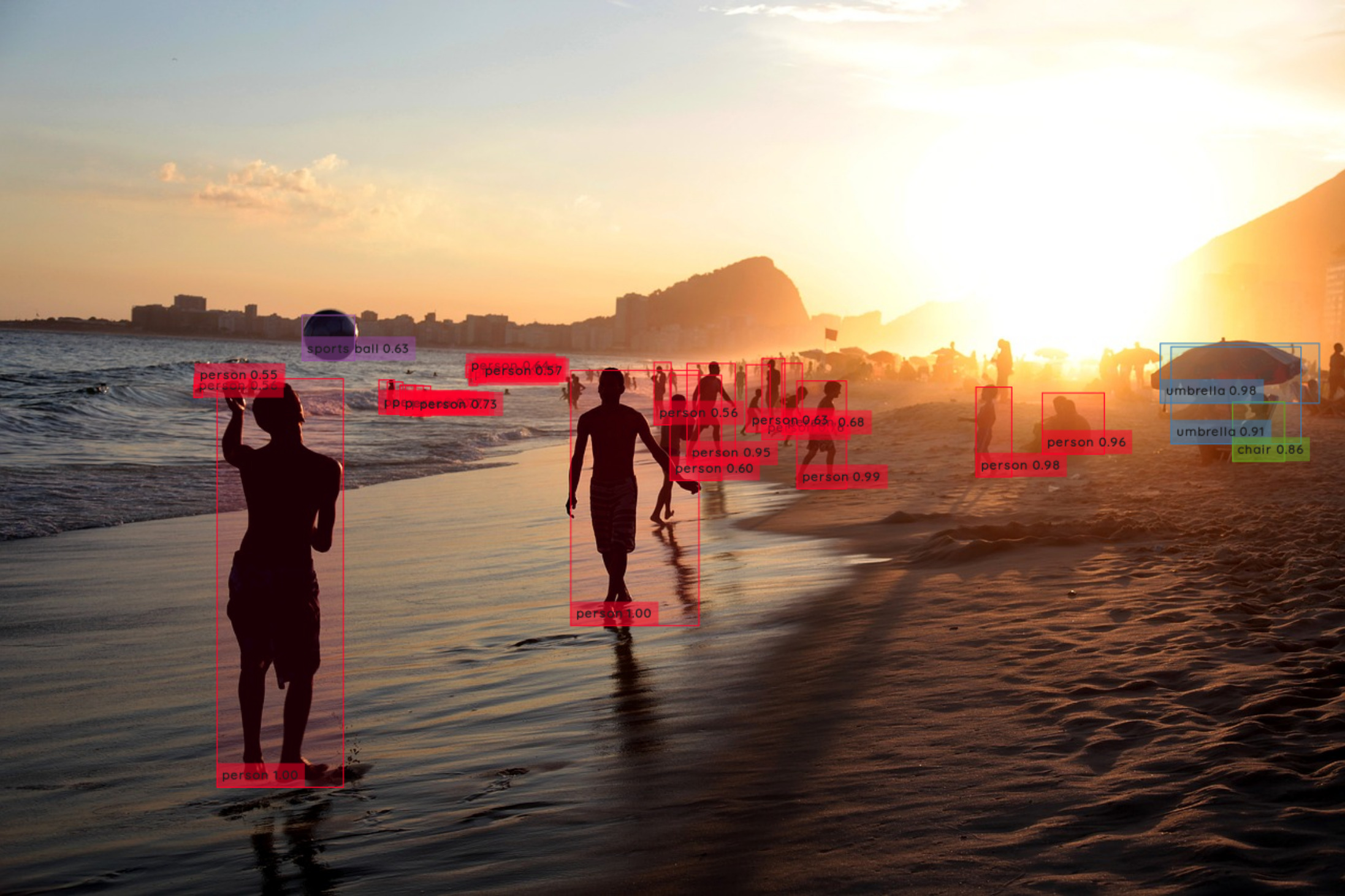
If we want Luminoth to predict the objects present in one of pictures (image.jpg). The way to do that is by running the following command:

1

lumi predict image.jpg

The result will be like this:

1
2
3

Found 1 files to predict.
Neither checkpoint not config specified, assuming `accurate`.
Checkpoint not found. Check remote repository? [y/N]:

Since you didn’t tell Luminoth what an “object” is for you, nor have taught it how to recognize said objects. So one way to do this is to use a pre-trained model that has been trained to detect popular types of objects. E.g., it can be a model trained with COCO dataset or Pascal VOC. What’s more, each pre-trained model might be associated with a different algorithm. The checkpoints correspond to the weights of a particular model (Faster R-CNN or SSD), trained with a particular dataset. The case of “accurate” is just a label for a particular Deep Learning model underneath, here, Faster R-CNN, trained with images from the COCO dataset.

After the checkpoint download, with these commands we can output everything (a resulting image and a json file) to a preds directory:

1
2

mkdir preds
lumi predict image.jpg -f preds/objects.json -d preds/

Exploring the Pre-trained Checkpoints

First, run the lumi checkpoint refresh command, so Luminoth knows about the checkpoints that it has available for download. After refreshing the local index, you can list the available checkpoints running lumi checkpoint list:

1
2
3
4
5
6

================================================================================
|           id |                  name |       alias | source |         status |
================================================================================
| e1c2565b51e9 |   Faster R-CNN w/COCO |    accurate | remote |     DOWNLOADED |
| aad6912e94d9 |      SSD w/Pascal VOC |        fast | remote | NOT_DOWNLOADED |
================================================================================

Here, you can see the “accurate” checkpoint and another “fast” checkpoint that is the SSD model trained with Pascal VOC dataset. Let’s get some information about the “accurate” checkpoint by the following command:

1

lumi checkpoint info e1c2565b51e9

or

1

lumi checkpoint info accurate

If getting predictions for an image or video using a specific checkpoint (e.g., fast) you can do so by using the –checkpoint parameter:

1

lumi predict img.jpg --checkpoint fast -f preds/objects.json -d preds/

Playing Around with the Built-in Interface

Luminoth includes a simple web frontend so you can play around with detected objects in images using different thresholds. To launch this, simply type lumi server web and then open your browser at http://localhost:5000. If you are running on an external VM, you can do lumi server web –host 0.0.0.0 –port to open in a custom port.

Building Custom dataset

In order to use a custom dataset, we must first transform whatever format your data is in, to TFRecords files (one for each split — train, val, test). Luminoth reads datasets natively only in TensorFlow’s TFRecords format. This is a binary format that will let Luminoth consume the data very efficiently. Fortunately, Luminoth provides several CLI tools for transforming popular dataset format (such as Pascal VOC, ImageNet, COCO, CSV, etc.) into TFRecords.

We should start by downloading the annotation files (this and this, for train) and the class description file.

After we get the class-descriptions-boxable.csv file, we can go over all the classes available in the OpenImages dataset and see which ones are related to traffic dataset. The following were hand-picked after examining the full file:

1
2
3
4
5
6
7
8

/m/015qff,Traffic light
/m/0199g,Bicycle
/m/01bjv,Bus
/m/01g317,Person
/m/04_sv,Motorcycle
/m/07r04,Truck
/m/0h2r6,Van
/m/0k4j,Car

Luminoth includes a dataset reader that can take OpenImages format, the dataset reader expects a particular directory layout so it knows where the files are located. In this case, files corresponding to the examples must be in a folder named like their split (train, test, …). So, you should have the following:

1
2
3
4
5

.
├── class-descriptions-boxable.csv
└── train
    ├── train-annotations-bbox.csv
    └── train-annotations-human-imagelabels-boxable.csv

Then run the following command:

1
2
3
4
5
6
7

lumi dataset transform \
      --type openimages \
      --data-dir . \
      --output-dir ./out \
      --split train  \
      --class-examples 100 \
      --only-classes=/m/015qff,/m/0199g,/m/01bjv,/m/01g317,/m/04_sv,/m/07r04,/m/0h2r6,/m/0k4j

This will generate TFRecord file for the train split:

1
2
3
4
5
6
7
8
9
10

INFO:tensorflow:Saved 360 records to "./out/train.tfrecords"
INFO:tensorflow:Composition per class (train):
INFO:tensorflow:        Person (/m/01g317): 380
INFO:tensorflow:        Car (/m/0k4j): 255
INFO:tensorflow:        Bicycle (/m/0199g): 126
INFO:tensorflow:        Bus (/m/01bjv): 106
INFO:tensorflow:        Traffic light (/m/015qff): 105
INFO:tensorflow:        Truck (/m/07r04): 101
INFO:tensorflow:        Van (/m/0h2r6): 100
INFO:tensorflow:        Motorcycle (/m/04_sv): 100

Training the Model

Training orchestration, including the model to be used, the dataset location and training schedule, is specified in a YAML config file. This file will be consumed by Luminoth and merged to the default configuration, to start the training session.

You can see a minimal config file example in sample_config.yml. This file illustrates the entries you’ll most probably need to modify, which are:

1) train.run_name: the run name for the training session, used to identify it.
2) train.job_dir: directory in which both model checkpoints and summaries (for TensorBoard consumption) will be saved. The actual files will be stored under /.
3) dataset.dir: directory from which to read the TFRecord files.
4) model.type: model to use for object detection (fasterrcnn, or ssd).
5) network.num_classes: number of classes to predict (depends on your dataset).

For looking at all the possible configuration options, mostly related to the model itself, you can check the base_config.yml file.

Building the config file for the dataset

Probably the most important setting for training is the learning rate. You will most likely want to tune this depending on your dataset, and you can do it via the train.learning_rate setting in the configuration. For example, this would be a good setting for training on the full COCO dataset:

1
2
3
4

learning_rate:
  decay_method: piecewise_constant
  boundaries: [250000, 450000, 600000]
  values: [0.0003, 0.0001, 0.00003, 0.00001]

To get to this, you will need to run some experiments and see what works best.

1
2
3
4
5
6
7
8
9
10
11
12
13
14
15
16
17
18
19

train:
  # Run name for the training session.
  run_name: traffic
  job_dir: <change this directory>
  learning_rate:
    decay_method: piecewise_constant
    # Custom dataset for Luminoth Tutorial
    boundaries: [90000, 160000, 250000]
    values: [0.0003, 0.0001, 0.00003, 0.00001]
dataset:
  type: object_detection
  dir: <directory with your dataset>
model:
  type: fasterrcnn
  network:
    num_classes: 8
  anchors:
    # Add one more scale to be better at detecting small objects
    scales: [0.125, 0.25, 0.5, 1, 2]

Running the training

Assuming you already have both your dataset (TFRecords) and the config file ready, you can start your training session by running the command as follows:

1

lumi train -c config.yml

You can use the -o option to override any configuration option using dot notation (e.g. -o model.rpn.proposals.nms_threshold=0.8). If you are using a CUDA-based GPU, you can select the GPU to use by setting the CUDA_VISIBLE_DEVICES environment variable.

Storing checkpoints (partial weights)

As the training progresses, Luminoth will periodically save a checkpoint with the current weights of the model. The files will be output in your / folder. By default, they will be saved every 600 seconds of training, but you can configure this with the train.save_checkpoint_secs setting in your config file. The default is to only store the latest checkpoint (that is, when a checkpoint is generated, the previous checkpoint gets deleted) in order to conserve storage.

Evaluating Models

Generally, datasets (like OpenImages, which we just used) provide “splits”. The “train” split is the largest, and the one from which the model actually does the learning. Then, you have the “validation” (or “val”) split, which consists of different images, in which you can draw metrics of your model’s performance, in order to better tune your hyperparameters. Finally, a “test” split is provided in order to conduct the final evaluation of how your model would perform in the real world once it is trained.

Building a validation dataset

Let’s start by building TFRecords from the validation split of OpenImages. For this, we can download the files with the annotations and use the same lumi dataset transform that we used to build our training data.

In your dataset folder (where the class-descriptions-boxable.csv is located), run the following commands:

1
2
3

mkdir validation
wget -P validation https://storage.googleapis.com/openimages/2018_04/validation/validation-annotations-bbox.csv
wget -P validation https://storage.googleapis.com/openimages/2018_04/validation/validation-annotations-human-imagelabels-boxable.csv

After the downloads finish, we can build the TFRecords with the following:

1
2
3
4
5
6
7

lumi dataset transform \
      --type openimages \
      --data-dir . \
      --output-dir ./out \
      --split validation  \
      --class-examples 100 \
      --only-classes=/m/015qff,/m/0199g,/m/01bjv,/m/01g317,/m/04_sv,/m/07r04,/m/0h2r6,/m/0k4j

The lumi eval command

In Luminoth, lumi eval will make a run through your chosen dataset split (ie. validation or test), and run the model through every image, and then compute metrics like loss and mAP. If you are lucky and happen to have more than one GPU in your machine, it is advisable to run both train and eval at the same time.

Start by running the evaluation:

1

lumi eval --split validation -c custom.yml

The mAP metrics

Mean Average Precision (mAP) is the metric commonly used to evaluate object detection task. It computes how well your classifier works across all classes, mAP will be a number between 0 and 1, and the higher the better. Moreover, it can be calculated across different IoU (Intersection over Union) thresholds. For example, Pascal VOC challenge metric uses 0.5 as threshold (notation mAP@0.5), and COCO dataset uses mAP at different thresholds and averages them all out (notation mAP@[0.5:0.95]). Luminoth will print out several of these metrics, specifying the thresholds that were used under this notation.

Using TensorBoard for Visualizing

TensorBoard is a very good tool for this, allowing you to see plenty of plots with the training related metrics. By default, Luminoth writes TensorBoard summaries during training, so you can leverage this tool without any effort:

1

tensorboard --logdir <job_dir>/<run_name>

If you are running from an external VM, make sure to use --host 0.0.0.0 and --port if you need other one than the default 6006.

What to look for

First, go to the “Scalars” tab. You are going to see several tags.

validation_losses

Here, you will get the same loss values that Luminoth computes for the train, but for the chosen dataset split (validation, in this case). As in the case of train, you should mostly look at validation_losses/no_reg_loss.

These will be the mAP metrics that will help you judge how well your model perform:

The mAP values refer to the entire dataset split, so it will not jump around as much as other metrics.

Manually inspecting with lumi server web

You can also use lumi server web command that we have seen before and try your partially trained model in a bunch of novel images. For this, you can launch it with a config file like:

1

lumi server web -c config.yml

Here you can also use –host and –port options.

Creating and Sharing Your Own Checkpoints

Creating a checkpoint

We can create checkpoints and set some metadata like name, alias, etc. This time, we are going to create the checkpoint for our traffic model:

1
2
3
4

lumi checkpoint create \
    config.yml \
    -e name="OpenImages Traffic" \
    -e alias=traffic

You can verify that you do indeed have the checkpoint when running lumi checkpoint list, which should get you an output similar to this:

1
2
3
4
5
6
7

================================================================================
|           id |                  name |       alias | source |         status |
================================================================================
| e1c2565b51e9 |   Faster R-CNN w/COCO |    accurate | remote |     DOWNLOADED |
| aad6912e94d9 |      SSD w/Pascal VOC |        fast | remote |     DOWNLOADED |
| cb0e5d92a854 |    OpenImages Traffic |     traffic |  local |          LOCAL |
================================================================================

Moreover, if you inspect the ~/.luminoth/checkpoints/ folder, you will see that now you have a folder that corresponds to your newly created checkpoint. Inside this folder are the actual weights of the model, plus some metadata and the configuration file that was used during training.

Sharing checkpoints

Simply run lumi checkpoint export cb0e5d92a854. You will get a file named cb0e5d92a854.tar in your current directory, which you can easily share to somebody else. By running lumi checkpoint import cb0e5d92a854.tar, the checkpoint will be listed locally.

Using Luminoth with Python

Calling Luminoth from your Python app is very straightforward.

1
2
3
4
5
6
7
8
9
10
11
12
13
14
15

from luminoth import Detector, read_image, vis_objects

image = read_image('traffic-image.png')

# If no checkpoint specified, will assume `accurate` by default. In this case,
# we want to use our traffic checkpoint. The Detector can also take a config
# object.
detector = Detector(checkpoint='traffic')

# Returns a dictionary with the detections.
objects = detector.predict(image)

print(objects)

vis_objects(image, objects).save('traffic-out.png')

The End

Hope you enjoyed the simple tutorial! :)

Computer-Vision, Object-Detection — Feb 14, 2020